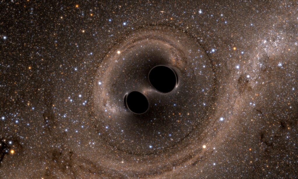
Everything consists of spacetime.
The first development steps for the DP were several different starting points. None of them was this approach, because we are building here. Over time, the various approaches have converged on this point. That was the point when a collection of loose ideas formed a theory.
The basic idea is the continuation of an ingenious thought by Einstein. If gravitation, as a purely geometric description, is mapped onto only one object, spacetime (spacetime curvature), then we must “simply” transfer this idea to everything else.
Since we start from the GR, we get the characteristic equation for the GR in its simplest form. Einstein’s field equations.
G_{\mu\nu}\space =\space k\space *\space T_{\mu\nu}
Let’s take a closer look at the structure of the equation.
The first thing that stands out: Why the field equations? There is only one equation. This notation is very compact. There are 16 individual equations, which together form a system of equations. The Greek letters μ and ν count from 0 to 3 (that is a convention). Each letter represents the number of dimensions in our space-time. According to the textbook, our space-time has 4 dimensions. Three spatial dimensions and one temporal dimension. In fact, there are 4 space dimensions in the equation. The time dimension gets an additional factor that turns time into length. The unit of measurement of the time dimension in the mathematical description is a length and not a time. The time dimension gets a different sign than the spatial dimensions. Space dimensions a plus and the time dimension a minus or vice versa. How this is done is purely a matter of opinion. What is important is that the signs are different. This is called the signature of space-time. We use the signature (- + + +). The capital letters are tensors. They describe how the content of the tensors behaves from one dimension to another. This results in 4 * 4 possibilities, 16 equations. However, due to symmetries, only 10 independent equations are needed.
Contrary to the textbook, we will only count the real space dimensions, i.e. those with +. Thus our space-time is 3D. Why we do this will be explained in chapter 3 “Borders”. We will see that this signature alone is not sufficient to classify space-time. The additional time dimension automatically results in any space-time configuration.
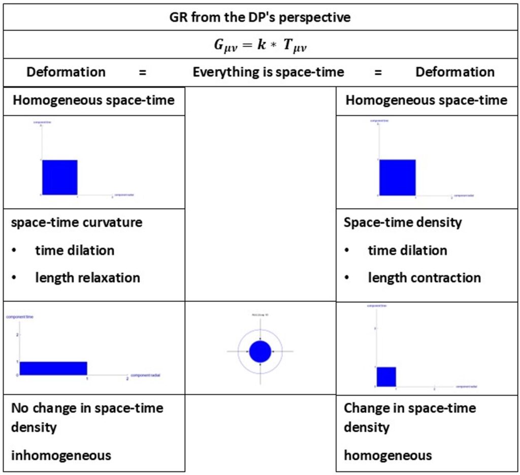
The left-hand side of the equation only has the tensor labeled G, the Einstein tensor. This describes, let’s call it quite generally, a deformation of space-time itself. This type of deformation is called the curvature of space-time. In GR, the curvature of space-time is equated with gravitation. Thus, gravity is not a force or an interaction, but a geometric mapping on exactly one single object, space-time. Our approach is to maintain a geometric identity across all considerations of an object. Thus, for gravity, the desired form of description has already been achieved. This immediately raises the question of whether we can do the same for the other side of the equation.
We transfer the idea of a mapping in space-time to the other side of the equation. There we have two elements. First, the small k. This is a proportionality constant. It contains only fixed values and thus, in the mathematical sense, represents only a fixed number with the appropriate unit of measurement. We will examine this k later. Then there is the energy-momentum tensor T. This contains everything that is known as the mass-energy equivalent. As with G, it is divided into the respective dimensions in relation to each other.
Without realizing it, the goal has already been achieved. It looks like the opposite. The energy-momentum tensor is a wild collection of everything the universe has to offer except for gravity. How can an equation with such a diverse collection of objects be so clearly represented? Because the collection is not as wild as it looks. If we look at the equation as a unification of GR and QFT, everything becomes clear. G describes gravity and T collects the entire particle zoo from the standard model, plus momentum, charges, etc. We know that the descriptions do not match, and yet we have an equal sign here. For this equation to work and for the difference to QFT to arise, GR must adopt a special view of this collection. The differences must be normalized. As always, this is done via energy. No matter how different the energy contributions from the energy-momentum tensor are, GR must adopt a normalized view. GR may only be interested in two things from T. The amount of energy and the possible alignment with the dimensions. Any “inner structure” of a mass-energy equivalent (is it an electron, photon, proton, etc.) must be hidden.
The Einstein tensor only uses spacetime with a deformation. We will do the same with the energy-momentum tensor. Certain requirements are placed on the geometric mapping in the energy-momentum tensor. The equation must continue to work and all statements of GR on gravity must follow from it. For some of the statements, the mapping to QFT must already fit at this level. That sounds like a very difficult geometric mapping in space-time. Exactly the opposite is the case. We will assume a “density” of space-time itself that is uniformly distributed in a certain volume of space-time. The deformation of space-time for gravity is called space-time curvature. We will now call the deformation of space-time, which is the source of space-time curvature, space-time density. In this case, “density” describes this deformation very well at certain points, but at other points it is rather a hindrance. We have to give it some name.
Force of sovereign arbitrariness => space-time density.
We will see that the consequences of this assumption will lead us to a complete description of physics. If someone had told me this before developing the DP, I would have thought that person was crazy. This approach has a great advantage for testing the DP. There is almost no choice for the conclusions. Either the logic and mathematics are correct or the whole theory collapses. There are only very few places where there is still room for “extensions”. The possibilities as in other theories, with smaller structures, higher energies, higher masses, further particles, etc., are not given here.
The only additional assumption to the known physics is the space-time density. What could possibly change? Almost everything, without really having to adjust the mathematics. As I said, it does sound a bit crazy.
We have invented the space-time density. So we should do two things first:
Let’s not make life more difficult than it is and start with something we already know. Space-time curvature has been known for over 100 years and is well understood mathematically. The space-time density is the source of space-time curvature. Thus, we can see space-time curvature as the reaction of space-time to space-time density. This behavior is described by the field equations. The definition of space-time density must agree with the solutions of the field equations already given.
In this text, we always use the solution of the field equations according to Schwarzschild. This has advantages but also disadvantages. The big advantage is that this solution is the simplest one. Schwarzschild found this solution only a few months after Einstein’s publication. This is a vacuum solution for non-rotating masses. We are sure that this is a strong simplification. But it is sufficient for our purposes.
To understand the solution, we have to write out the signature of spacetime (- + + +) in full. The signature is just a shorthand form of a metric. The metric of spacetime defines the behavior of spacetime with respect to the field equations. If you will, the metric is the solution of the equation. 4 x 4 entries for all the different divisions between the dimensions. Extremely important for us: the metric is the appropriate definition of the geometry for space-time. Schwarzschild metric:
\begin{pmatrix} -c^2(1\space -\space \cfrac{r_S}{r} )dt^2 & 0 & 0 & 0 \\ 0 & +\space \cfrac{1}{(1\space -\space \cfrac{r_S}{r})}dr^2 & 0 & 0 \\ 0 & 0 & +\space r^2d\theta^2 & 0 \\ 0 & 0 & 0 & +\space r^2sin^2(\theta)d\phi^2 \end{pmatrix}
Don’t panic, it looks worse than it is. In the diagonal of this matrix, you can see the signs from the signature (- + + +) first. Behind them, however, there is a term in each case. The last two terms with \theta or \phi are not relevant to us at the moment. This solution is based on spherical coordinates. The last two terms indicate the position on a spherical surface. Like longitude and latitude on the earth’s surface. However, we are only interested in the distance, i.e. the radius of this spherical surface, and not the position on it. Fortunately, in spherical coordinates, the effect of gravity only depends on the distance. This means that only the first two terms are still relevant.
The first term is the time dimension. This can be seen from dt^2 and the minus sign. However, this term is multiplied by a c^2. The speed is a length divided by time and the time dimension is only a time. After shortening, only a length remains. The time dimension is converted into a space dimension in the mathematical consideration. There are 4 space dimensions. We stick with the designation from the textbooks and still say time dimension. The small r is the distance from the source of gravity and the r_S is the Schwarzschild radius. The event horizon of the black hole.
The second term is the radial distance to the gravitational source. You don’t have to be a mathematical genius to realize that the second term is the reciprocal of the first term. This means that time and space dimensions behave to the same extent but in opposite directions. If you are far away from the source of gravity, then the distance r of r_S is large and the fraction approaches zero. Thus, there is only one 1 in the parenthesis and we have a flat spacetime and no gravity. However, gravity never becomes exactly zero. This means that gravity has an infinite range. If you approach r_S, then the fraction approaches 1. At the Schwarzschild radius, this is exactly 1. At the time dimension, the parenthesis becomes zero. The time dimension then no longer has any extension/length. Time stands still for a distant observer. At the radial space dimension, the parenthesis also approaches zero. But at zero, the division by zero results in a singularity. A value of infinity, or better, not defined. This is another disadvantage of the Schwarzschild metric. This singularity does not occur at the event horizon with other metrics. It can be shown that this is only a peculiarity of this metric, a mathematical artifact. Since the parenthesis is in the denominator with the radial component, the expansion/length before the Schwarzschild radius approaches infinity.
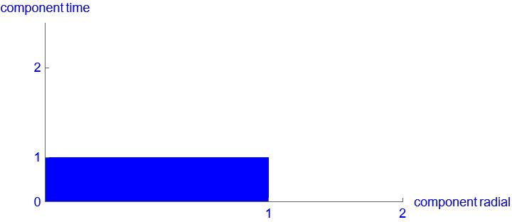
If the time and space dimensions form a rectangle, the following occurs:
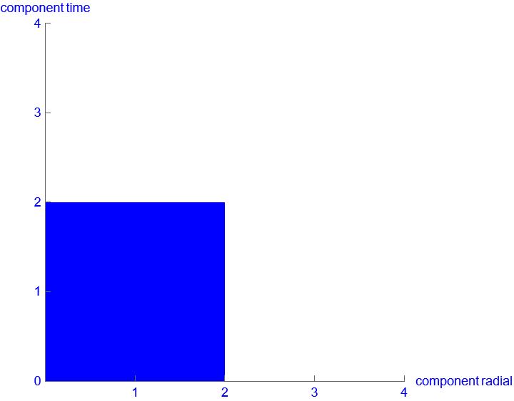
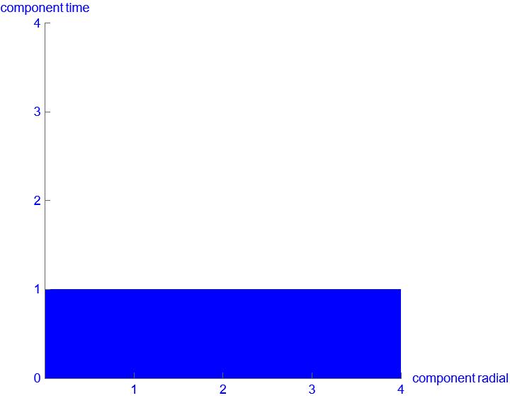
Figure 01 is a spacetime without spacetime curvature. In Figure 02, the time component corresponding to a space component is shortened and the radial space component is lengthened.
The time dimension becomes smaller and the space dimension larger to the same extent. The crucial point in the consideration is that the area of the rectangle does not change. If time is halved, the length doubles => identical area. This consideration of space-time curvature is sufficient for us to be able to justify our space-time density.
Let’s stick with a spherically symmetric example. If the radial space component in the direction of the gravitational source is getting longer and longer, where does this additional length go? What you often hear is: into the space-time curvature. We want to describe the space-time curvature as a reaction to the space-time density. Therefore, we reverse the argument. It is easier if we assume that the space-time of the gravitational source has shortened with some deformation. Space-time curvature must compensate for this with additional length. We continue to assume that space-time is a continuum. If you will, because of the continuity of space-time, space-time curvature fills the missing expansion of space-time to space-time density.
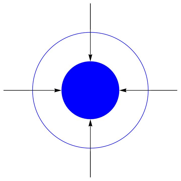
Figure 03: The space-time density has “condensed” the space-time in the circle towards the disk. In the space-time volume (circle), the space-time curvature (arrows) must “push” space-time into this volume through space-time curvature so that the space-time to the space-time density (disk) remains a continuum.
We are considering a volume of spacetime and still have the spherical coordinates. However, in the case of a volume of spacetime, not only one length may become shorter due to deformation. The entire volume of spacetime of the gravitational source must become smaller. We continue to assume that space-time behaves identically when deformed. Then, in addition to the radial spatial dimension, the temporal dimension must also change to the same extent. Not in the opposite direction, otherwise we would not get a smaller volume. In this case, the temporal dimension must shorten to the same extent as the spatial dimension.
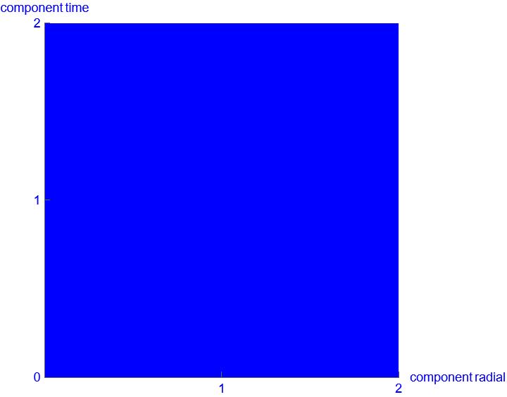

Figure 04 shows a spacetime without spacetime density. In Figure 05, the spacetime must “condense” into a smaller volume.
The deformation of space-time for the gravitational source looks like a “density”. The previously larger area must now be accommodated in a smaller area.
Hence the name: space-time density
How should we visualize this density? With a material such as a sponge, you can easily recognize its density by squeezing it. Does the same thing happen with space-time? Definitely not! When it comes to density, it is helpful to think of a substance. In a substance, you can recognize the density from the outside and also determine it within the substance itself. As with the sponge. But space-time can be deformed. Space-time curvature, space-time density, expansion, twisting of space-time around a black hole or gravitational waves, it all sounds a lot like a changeable substance. This analogy is like the word density. Sometimes it fits and sometimes it doesn’t. Right here, neither substance nor density fits. Because nothing is “squeezed”. We have simply shortened the lengths in the images above. That does not happen. What really happens is that the definition of geometry has changed.
We redraw the two images of space-time density with the correct divisions on the coordinates. Then it looks like this:


Figure 06 shows a spacetime without spacetime density. Figure 07 has a different scale. Here the unit length from 0 to 1 in the spacetime density is defined differently than outside the spacetime density, e.g. from 1 to 2.
See the difference. The step of a unit of length remains a 1 in both pictures. What has really changed here is how a meter is defined for the spatial dimension and a second for the temporal dimension. This only applies within the space-time density. This means that in each rectangle the area is 1. No change locally. Only by comparing the rectangles can you see that the definition of time and length must be different.
The spacetime density is actually a “density of the definition of the geometry of spacetime” or a “density of spacetime definition”. These are long names or obscure abbreviations. We’ll stick with spacetime density. In old versions of DP or in the videos on the YouTube channel “Dimensionale Physik”, I tried to introduce the abbreviation DRD for Density of Space-Time Definition. Just forgot about it again, sorry about that.
Five times in bold “Definition”. I hope that has stuck. Nothing is condensed like a substance. In the metric of space-time, there is no classical stretching or density. The definition of what the unit of length 1 meter or the unit of time 1 second is, is changed. This shorter definition is the higher density. Only with the perspective of the definition can we later build a relativity principle in which no change can be detected locally.
We can also do this with the sponge.
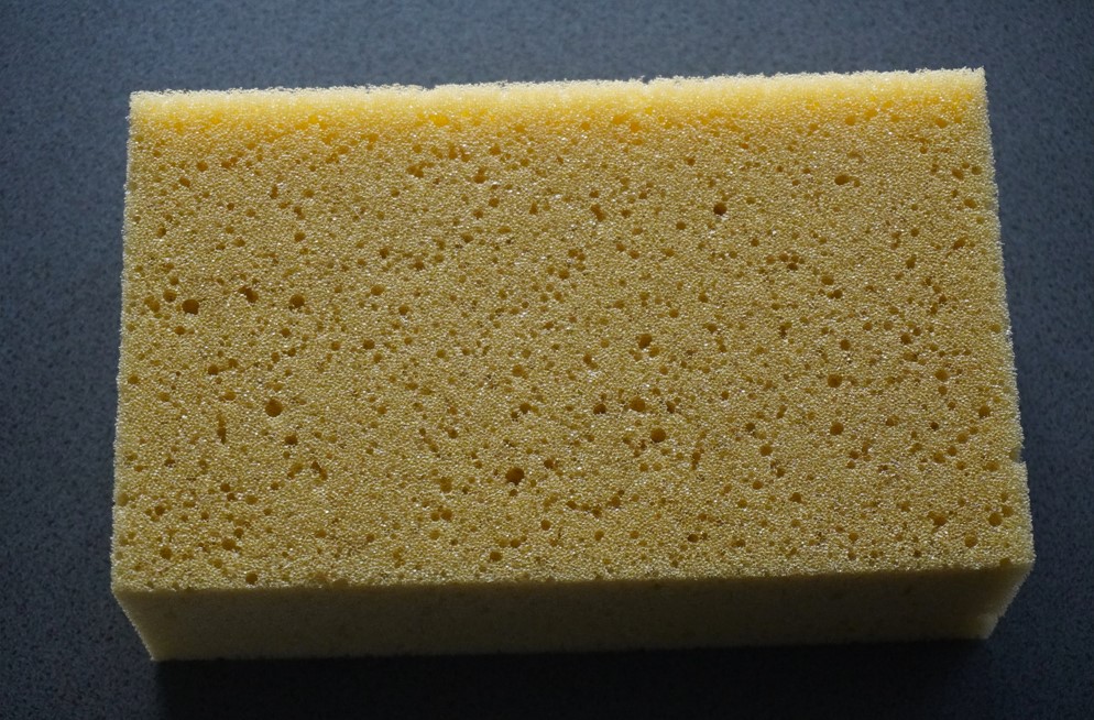
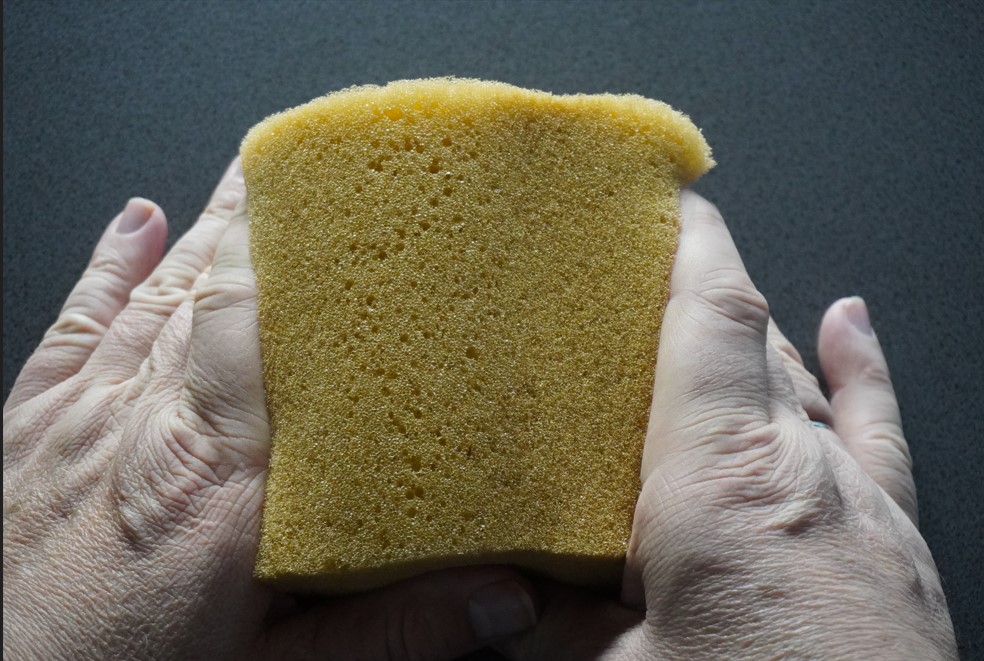
Figure 08 and Figure 09 do not show space-time, but a substance. The sponge as a substance with more density.
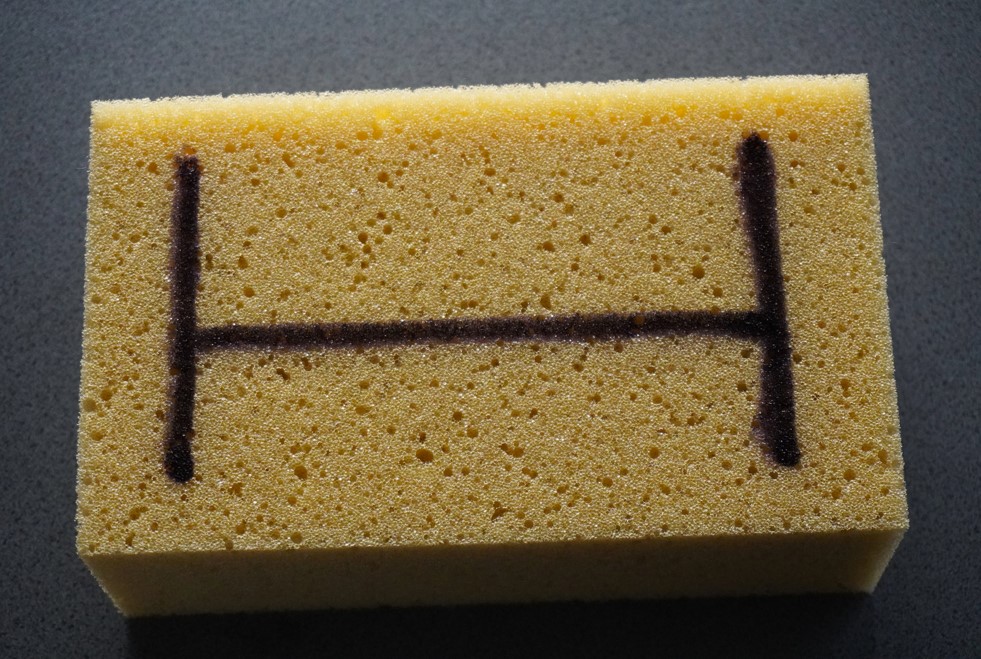
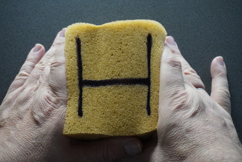

In Figure 10, we have to imagine the sponge as gone and only see the black line as the length definition. In Figure 11, only the length definition (without the sponge) has been changed.
What has just been said about the density of space-time also applies to the curvature of space-time. Here is the curvature of space-time with the correct divisions when drawing:

In figures 12 and 13, the space-time curvature is to scale.
There are still more names to define. In the SR, the individual components have been found to be length contraction and time dilation. We will continue to use these terms exactly as they are. For the space-time density on the time dimension, time dilation and on the space dimension, length contraction. When space-time curvature occurs, the time dimension is also defined as becoming smaller, so this is also time dilation. However, there is no separate term for the change in the spatial dimension when space-time is curved. Here, the term space-time curvature is often used directly. From now on, we will use space-time density and space-time curvature only for the behavior of the entire space-time. To keep the same syntax, we will use the term length relaxation for the change in the spatial dimension when space-time is curved.
Every individual, every planet and even every elementary particle is a spacetime density in just a single object, spacetime. This is continuous. There are no boundaries within spacetime. According to DP, we are all together and, physically speaking, we are just different spacetime densities in a single spacetime. This approach is probably the strongest collective thought we can apply.
The QFT will have a slightly different opinion on this. For the ART, however, this is 100% correct. We should always have this collective thought in mind when dealing with other individuals. According to DP, this is always a way of dealing with ourselves. The thought is as beautiful as it is frightening.
At the end of this chapter, we want to test our assumption of spacetime density at a high level. We just have to be able to explain the behavior of the GR based on the geometry. The mathematics, the how, is not changed. Our goal is to be able to explain the why of the mathematics. The assumptions that led to the SR and GR the principle of relativity, the speed of light and the equivalence principle will be discussed in separate chapters. This will be the real test. We have to be able to generate these assumptions from our approach. We cannot reuse them, otherwise we get a circular argument. The starting point was already the GR. Let’s go through a few points.
For us, spacetime curvature is the reaction of spacetime to spacetime density. Since the spacetime density “contracts”, spacetime as a continuum must compensate for this. Spacetime curvature must necessarily align itself in the direction of spacetime density. In the first approach, spacetime density has no direction. A density can be described as being evenly distributed over the volume.
We can rearrange the field equations. We put the Einstein tensor on the same side as the energy-momentum tensor. This transformation is allowed for any equation.
0\space =\space k\space *\space T_{\mu\nu}\space -\space G_{\mu\nu}
Now, the space-time density and the space-time curvature must cancel each other out. A change in sign for a geometric figure is always a change in direction. Thus, the space curvature now pulls away from the space-time density. The space-time density is now “pulled apart” by the space-time curvature (the condensation dissolves). This is no change for the space-time in total, so it is equal to zero.
To do this, let’s take another look at Figure 03. Memorize the image well, we will need it again and again.
We see that the space-time curvature deforms the space-time towards the space-time density. Thus, the space-time outside the ring must be pulled/deformed towards the space-time density. Space-time is a continuum and must not “tear”.
If something deforms in one direction, then the neighboring area must also deform in this direction. Then the neighboring area of the neighboring area must deform, and so on. Therefore, the space-time curvature must have an infinite range.
The effect of gravity decreases with distance. This must decrease more steeply than linearly. With distance, away from a space-time density, the space-time curvature can access an ever-increasing space-time volume that must deform with it. Therefore, the weakening in our 3D space-time must occur with the square of the distance. In the opposite direction of gravitation, one spatial dimension 1D is added to an increase in volume of two spatial dimensions. If we consider the blue ring as a spherical shell in 3D, then we can place ever larger spherical shells around the space-time density. The radius of the area on which gravity acts grows linearly. However, the area grows with r^2.
We continue with Figure 03. We can see that the space-time must “push” towards the space-time density with the space-time curvature. The space-time must compensate here. Then it only makes sense for the space-time if the pushing-in by the space-time curvature is done in such a way that the space-time density of the surrounding space-time is not changed by the space-time curvature up to the gravitational source. The space-time curvature must therefore be a deformation of the space-time that itself does not produce any change in the space-time density. From the approach with the space-time density, the space-time curvature must show the known behavior (area remains the same).
We continue with Figure 03. We can see that the space-time must “push” towards the space-time density with the space-time curvature. Spacetime must compensate here. Right! The beginning repeats itself. This is not a mistake. We need the statements again here.
Spacetime curvature must compensate for the gap between the ring and the disk. But this also means that spacetime curvature must explicitly not compensate into the spacetime density. For spacetime curvature, the end is reached at the boundary of the spacetime density. There is already too much space-time in the space-time density. The space-time curvature must not reach into it and make the problem worse.
Important! The space-time curvature is not there to balance the space-time density. Due to the continuity of space-time, the space-time density must compensate for the missing length to the space-time density. Space-time curvature is not supposed to dissolve space-time density. For space-time curvature, only the amount of space-time density is of interest, since a larger space-time density means that a larger gap has to be filled. Whether space-time density has an “inner” structure is completely irrelevant for space-time curvature and thus for GR. QFT will then describe precisely this “inner” structure.
Spacetime curvature is a compensation for a “spacetime gap” caused by the spacetime density. The spacetime density itself is not changed by spacetime curvature. Spacetime curvature ends at the boundary of the spacetime density. Here you can already see how we get rid of the singularity in GR later. A space-time density without a space-time volume makes little sense. No volume, no density, no gravity, and thus no singularity due to gravity. We will discuss the mathematical abstraction of a point and thus the singularity in detail in Chapter 3, “Borders of Space-Time”.
We continue with Figure 03. We can see that the spacetime must “follow up” with the spacetime curvature to the spacetime density. The spacetime must compensate here. Yes, again!
What we can also see is that the spacetime has condensed in a circle through higher spacetime density onto the disk. The space-time density itself is irrelevant for the GR in the disk. The amount of space-time density determines the size of the disk and this is what space-time curvature is interested in. Thus, the space-time density in the disk can be assumed to be uniformly distributed. The description of the space-time density can thus be done in a linear description. This will be one of the reasons why the QFT can be described linearly.
This is not the case with the GR. Space-time curvature does not change the space-time density when it is curved. However, as we can see, space-time “pushes” further space-time towards the space-time density due to space-time curvature. This means that the space-time density in the circle has increased again due to space-time curvature. This gives us a self-reinforcing effect. The mathematical description of GR must not be linear under any circumstances.
All physicists hope that if GR is unified with QFT, GR can possibly also be described linearly from a QFT approach. Linear descriptions are easier to solve. In QFT, the description is linear but extremely complicated from the ground up. It is only because this is a linear description that anything can be calculated at all. The description of GR is not that complicated and is mathematically very well understood. Unfortunately, however, GR is not linear. Thus, in both areas, the supercomputers are busy calculating approximate solutions.
Finally, we select a topic that does not belong to GR. We want to see that the density approach also works in other areas of physics. For this, we select something that exists in many different forms. We want to cover a wide spectrum. In addition, we choose something where no one sees a problem. The point of view in physics should change fundamentally. This also means areas that have supposedly been ticked off as “understood”. The choice has fallen on the binding energy.
The binding energy exists in the atomic nucleus, the atomic shell, between atoms or molecules. Even the release of energy, when two black holes merge, can be explained according to this scheme. The whole structure has less energy than the individual parts before the bond. As an example, we take the fusion of hydrogen to form helium. There are several processes in the sun by which hydrogen turns into helium. We simplify the process a lot. This is sufficient for our purposes.
We assume that hydrogen H_1 turns into hydrogen H_3 and that this then fuses into helium H_4. We are only interested in the end result, the helium nucleus.
QFT calculates the exact probability of this fusion and the energy that must be released for it to occur. The form in which the energy is released is not relevant here. We start our game of questions: Why? Then you often get two answers.
Unfortunately, these are not answers to the question. Why a stable energy level, entropy? We could play the question-and-answer game for a long time here. What is important for us is that:
mathematics is a consistent description of nature through an appropriate model. We can use this model to make investigations and conjectures. However, mathematics will never create or enforce anything in real nature! The question why must clarify this and the model description can then provide a suitable how.
How do we explain this with space-time density? The two H_3 building blocks must be in close proximity for a bond to form. Bonding only works at close range. In this case, the two building blocks must come close enough for the strong nuclear force to have an effect. We will clarify the exact process of which nucleons are allowed to react with each other later in QFT.
Here, the point is that in the end result, 2 protons and 2 neutrons form a helium nucleus. To illustrate this, textbooks often use a sphere for each nucleon. We will try to do the same here. We will ignore the fact that a proton or a neutron itself is a composite system.
Now we know that the helium nucleus does not look like that at all. Experiments have shown that an atomic nucleus must look more like a single sphere with bulges. The calculations of QFT confirm this. How do we get from 4 individual nucleons to a sphere that is not much larger than the individual nucleons? Fortunately, we have our space-time density.
A spacetime density is not a structure with a closed boundary. Everything is spacetime. This means that individual spacetime densities can overlap. Therefore, bonds only work within a certain spatial proximity. To us, the helium nucleus looks more like this.
The individual nucleons are a space-time density. A space-time density can overlap. Each individual nucleon has too much space-time density with the overlap to be a proton or neutron. In order for the nucleons to remain at their level of space-time density, some of the space-time density must go away. There is too much of it! The nucleons do not want to go to a lower energy level. The nucleons must remain at their fixed energy level. If we want to break this nucleus down into its component parts, we have to add the missing space-time density. This is how the space-time density approach explains the binding energy very simply. There is a small overview of the binding energy.
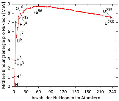
Figure 17 shows the binding energy per atomic nucleus. The horizontal axis is the number of nucleons in the atomic nucleus. The vertical axis is the average binding energy per nucleon [MeV]
source reference: https://lp.uni-goettingen.de/get/text/6933
As we can see, the binding energy increases very sharply with a few nucleons. This makes sense, since at the beginning a new large intersection of the space-time density is created with each individual nucleon. The more nucleons already present in the atomic nucleus, the smaller the new intersection between the space-time densities.
At a certain number of nucleons, the binding energy can drop again. The repulsion due to the charge ensures that the nucleons cannot overlap arbitrarily. Therefore, the geometry of the overlap can also cause less binding energy when a new nucleon is added. With iron Fe_{56}, that’s it. Each new nucleon causes a smaller intersection due to the change in the intersections between the space-time densities.
In addition, there are so-called “magic numbers” 2, 8, 20, 28, 50 and 82. These numbers of nucleons seem to have a very stable bond. According to QFT, when the atomic nucleus is “deformed”, these numbers result in an almost exact sphere for the entire atomic nucleus. A smooth sphere as a whole has the highest possible intersection of nucleons.
As we can see, with the approach of a space-time density, we can also explain the why in areas outside of the GR. With that, we will close this chapter and look at the most important conclusion from the space-time density.