Everything consists of spacetime.
In this chapter, we will derive the most important conclusion from the assumption of space-time density. Our space-time and every other space-time has limits. These limits have nothing to do with size, length or volume. These result from one more or less space dimension in a space-time. This will lead us to two conclusions that could not be more different in their statements.
These conclusions arise compellingly from the boundaries of spacetime. We have to live with the consequences, whether we like them or not. Cosmology is given its own chapter in Part 2 and QFT is in Part 3. This chapter is only about the boundaries and structure of our spacetime. That is already enough for a chapter of its own.
We already had a brief mention of spacetime as an object or substance in the last chapter. Since Einstein, it has been a popular point of contention as to whether spacetime is something real or just an abstract mathematical consideration. To better understand the approach with the density, let’s choose the idea of substance or, better yet, as a single object. The best argument in favor of substance is the expansion of spacetime.
Example: If the space between our galaxy and a distant galaxy is only a mathematical abstraction, then the galaxies must move away from each other at faster than the light speeds from the Hubble horizon. If we want to prevent a speed faster than light for objects with a rest mass, then space-time must not be a pure mathematical abstraction. If distance and thus space-time are only an abstraction, we cannot decompose the motion of objects into different areas. This can only be avoided if space-time expands as a substance. The speed of light is then not in the space-time (abstract distance), but the space-time itself has this state of motion. This is not a problem for the GR. As I said: curvature, density, expansion, rotation of a black hole and gravitational waves. Our space-time seems to be very “malleable”. That must actually be a substance. However, there are places where we have a problem with this analogy:
The points can all be resolved by the fact that space-time defines the geometry and thus determines whether a length or time exists at all. Outside of a space-time, no geometry exists. Space-time is a separate object class in itself. To better understand the argument, we start from the analogy of a substance.
When examining a description, one often starts with the following consideration: What happens at zero or at infinity? We look at the extreme of a space-time density.
Case 1 => infinity: The time and space dimensions approach zero uniformly. Thus, the space-time density increases and approaches infinity. Since both dimensions approach zero, the increase in space-time density must be at least quadratic. In addition, there must be a non-exceedable limit for the “shrinkage” of the time and space dimensions. When we reach zero for the dimensions, that’s it. It can’t go any further. Shortly before this limit, however, the space-time density approaches infinity.
A space-time density that occupies all three spatial dimensions of our space-time can never reach this limit. A given spatial dimension cannot simply disappear. We would have to be able to create an infinite space-time density. We will see that a space-time density of zero or infinity makes no sense. The reverse conclusion: A space-time density that occupies only two space dimensions and is not subject to any interaction must always be located at precisely this uncrossable boundary. Here, a space dimension cannot simply be created. The absence of a space dimension is the defining characteristic of this boundary. This means that there can be space-time densities that are not infinitely large but still exist at this boundary.
What we need is now clear. An absolute boundary that cannot be reached by certain objects and is the condition for existence for others. In addition, we need time dilation towards zero and length contraction towards zero. We know this, exactly the speed of light. We will see that the speed of light belongs to the structure of space-time and is therefore one of the most important natural constants of all.
Case 2 => zero: We want the space-time density to approach zero. For this, the time and space dimensions must let their definition of length and time approach infinity. Time relaxation and length relaxation. We had defined these names as such. This “countermovement” to the space-time density will be important again in the chapter on cosmology.
In this chapter, this statement is interesting. We do not get a boundary. The space-time density decreases, but will never become zero. This means that the existence of a space-time point is always connected with the existence of a space-time density.
According to the textbook, the speed of light c is the fixed maximum speed in our space-time. Thus, it has always been a boundary. What is so special about the DP’s point of view? This limit is a special limit. Let’s take a closer look at the speed of light.
As the name suggests, the speed of light is a speed. This is defined as \frac{length}{time}. What numerical value the speed of light has is purely arbitrary. We have defined the specification of one meter and one second and thus the value of the speed of light. Since it is generally accepted that the speed of light is a limit, in physics the definition is reversed. The speed of light is determined and a definition of meter and second is derived from it. From the point of view of DP, the speed of light can be determined very easily. This is the speed at which time dilation and length contraction reach zero. Thus the maximum deformation of space-time for a space-time density.
Why do we get a specific value for the speed of light? It should then be \frac{length = 0}{time = 0} for the object. This is an undefined mathematical expression and not a specific numerical value. Fortunately, our space-time has more than one spatial dimension. The mapping of the space-time density of an object moving at the speed of light can therefore only exist in the other two spatial dimensions. A space-time density must be mapped there, otherwise the object (e.g. a photon) would not be recognizable.
We already know that it is the Planck length and Planck time. But from the definition, there are infinitely many values for length and time. The speed is a fraction. It could also be, for example, only half the Planck length and half the Planck time. The boundary condition explicitly does not set Planck time and Planck length as the smallest possible length and time unit in space-time. It is the combination, i.e. the fraction, that makes up the speed of light. The important result for us is that although it is the boundary condition for our space-time with one less spatial dimension, it is still present in our space-time.
An observer recognizes (e.g. for a photon) a movement of the space-time density in the direction of movement with its time exactly on this boundary. For the space-time density, which moves at the speed of light, this definition says something different. If an object exists that has only mapped its space-time density onto two spatial dimensions, then this object cannot perceive our 3D space-time. One spatial dimension must be explicitly missing. But not just one spatial dimension. The temporal dimension is also missing. Like the spatial dimension, this tends towards zero. In the previous interpretation of this fact, it was not seen as anything special. For us, it is different.
One of Einstein’s greatest innovations was to combine space and time into a single object: space-time. Only in this way could the SR and later the GR work. We take this “unity idea” of space-time 100% seriously and apply it to the speed of light. If we want to leave our space-time, then time dilation must go to zero. This is an essential part of space-time. We have time dilation to zero at the speed of light. Now the behavior of the space-time components makes sense. Due to the length contraction, one spatial dimension becomes “less and less or denser”. You change the space-time configuration in the direction from (-, +, +, +) to (-, +, +). In the process, the time dimension also approaches zero due to time dilation and the result is (+, +). This is no longer space-time. There is no time dimension. We have thus left our space-time. From this consideration, we draw our most important conclusion. Our and thus all space-times have boundaries. These are defined by the fact that the time dimension approaches zero.
A space-time has boundaries
We already know one of these boundaries, the speed of light. This is the lower-dimensional boundary. Due to length contraction, we lose one spatial dimension at the speed of light. Thus, we change the spacetime configuration of spacetime and leave our spacetime. This is where the analogy with a substance is wrong. If you change the properties of a substance or an object, it is still the object. Only with different properties. In spacetime, it is different. If we change the spacetime configuration, one spatial dimension more or less, then we leave the spacetime.
Wait a minute! Now you have to object. In our space-time, we know objects that move at the speed of light. How can we recognize these objects if they are no longer in our space-time? We have already answered these questions. Because these objects have a space-time density that can only be mapped onto two spatial dimensions in our space-time. This means that such an object must move at the speed of light, instantly and without any delay, from the moment of its existence. Then, for example, a photon is a real interface object of our space-time. It lies directly on the boundary of space-time. It is only because the images of the space-time density are present on the other two spatial dimensions that we can recognize these objects at all. But then only in the state of the speed of light.
The speed of light is the lower-dimensional limit
I am personally very pleased with the realization that space-time has limits and that one of them is the speed of light. A long, long time ago, when I was at business school, I had a physics teacher, Mr. Werner. He fulfilled 100% of all prejudices and clichés for a math and physics teacher. Unfortunately, Mr. Werner died before I left school. Towards the end of my first year at school, some of the class sat around a campfire with a beer. It is important to me to emphasize that something like this did not happen during school lessons. Since I was already interested in physics, I asked Mr. Werner how he came to study physics and how he felt about it. He didn’t really get on with QM, but found GR very clean and beautiful. However, he had a problem with one point. This was not the singularity. Why is there this maximum speed that we know as the speed of light? Relativity and equivalence principle seemed logical and easy to understand to him. It was clear to him that all this only works if there is this maximum speed. However, the postulate of the speed of light seemed to him to be a “foreign body” in the theory. He would like to have a logical explanation for this.
This question from Mr. Werner has been on my mind ever since that evening and is one of the main reasons why the DP exists. With the approach of space-time density and space-time as an object/substance, this question is answered. The speed of light is not a fixed speed limit. This is a necessary consequence of the approach. There is no “higher” state of motion than the speed of light. The time and space dimension is zero. You can’t get less than that. You have to reverse the definition of the speed of light. It is not at the speed of light that time dilation and length contraction become zero. Reaching the lower-dimensional limit of our space-time is the condition for the definition of the speed of light.
The speed of light is a structural element of space-time
There is no reason for a postulate of the speed of light. This automatically results from the approach of the space-time density for a mass-energy equivalent.
It’s nice that I’ve found my personal peace with the low-dimensional limit. Does this realization help us in other ways? If I ask that question, yes. The low-dimensional limit or speed of light can be chosen as an identical term and explains the hard switch between objects with or without rest mass and what energy is.
As we approach the lower-dimensional boundary, the space-time density approaches infinity. We know the identical behavior from energy. This is no coincidence. In the DP, we equate space-time density and energy. This should be clear from the approach. We have set the space-time density as the source of space-time curvature. The source of space-time curvature is any form of energy. Therefore, the identity between energy and space-time density must necessarily result. But with this, we can explain what energy is. Energy and gravity are another way of defining the geometry of space-time itself.
Energy is the density of the geometric definition of space-time
To deepen this consideration further, we get the most famous formula of Einstein:
E\space =\space mc^2
The formula is correct. However, it is only so well known because the formula is very simple in this form. The complete formula never had a chance to become as well known because it is a bit more complicated:
E\space =\space \sqrt{m^2c^4\space +\space p^2c^2}
If the second term under the root is zero, we can take the root and end up with the familiar part again. For the second term to be zero, the momentum, i.e. the momentum with p^2, must necessarily be zero. The speed of light c is constant and cannot be zero.
The first term corresponds to the rest mass. We will not go into this in more detail. Why rest mass exists at all is a little more complicated. For this we need the complete part 3, the QFT.
The part of the rest mass that is of interest to us is that it is a scalar value. The rest mass does not depend on a direction.
We want to look at the second term, the momentum. This means that momentum must also have a direct mapping in the space-time geometry. The whole thing with a direction. For us, this means that there is a space-time density with an oriented direction.
For the colloquial term of density, an special direction sounds a bit strange. In a gas or a liquid, the density is identical in all directions. For spacetime, this is different. Here we only have the definition of geometry for a description. The spacetime density always lies on the time dimension and on at least one space dimension. We will explain why this is so in the section for time. The spacetime density does not necessarily have to be mapped on all space dimensions. We need at least one space dimension, otherwise the term spacetime density makes no sense. This means that a spacetime density with an oriented direction must be an impulse. With angular momentum, the direction is constantly changing, which means a constant change in geometry. We can detect this as a force. However, the spacetime density does not decrease. This is only shifted to another “direction/space dimension”.
If energy is directed in one spatial dimension and is therefore a momentum and thus a state of motion, then scalar energy, like rest mass, must also have a state of motion. Ok, but in which direction is the motion directed? In all directions simultaneously. We will see in the chapter on cosmology that this is the case, for example, with the expansion of space. Here we can define the following condition:
space-time density is energy, geometry of space-time and state of motion
Space and time were combined into one space-time. We must also do this for these terms. These terms are different descriptions of a single object, the space-time density.
A final word about movement. This is defined as follows in DP. If only one spatial dimension changes and the rest remain unchanged, we get a movement in space. This is what we colloquially describe as movement. If all spatial dimensions change mutually, then this is a change of the space itself. In the case of space-time curvature, the movement in space is changed, “equivalence principle”. If all spatial components change identically, space itself moves. This later results in the expansion of space-time. The differences are explained at the respective point.
With the previous picture of the space-time density, it is very easy to explain why there are objects with rest mass and a state of motion below the speed of light and objects without rest mass and the exact state of motion at the speed of light.
For an object with rest mass, e.g. an electron, the space-time density must occupy all three spatial dimensions of our space-time. The speed of light is the lower-dimensional limit of space-time. Our space-time loses a spatial dimension. A given spatial dimension cannot simply disappear. It can only receive an ever-increasing directed space-time density up to the speed of light. The scalar space-time density, for example for an electron, becomes more and more dense in the direction of motion. This results in an increasing energy up to infinity. This excludes the achievement of the speed of light.
Space-time density with rest mass = 3 space dimensions are occupied
An object without rest mass may not occupy all three space dimensions under any circumstances. It may only occupy two space dimensions. This means that one space dimension is already missing due to the “internal structure” of the object. The object must not experience any acceleration. It must already be moving at the speed of light from the moment of its existence. Another state of motion is not possible without interaction. The object lives in the low-dimensional interface of our space-time.
Space-time density without rest mass = 2 space dimensions are occupied
From this point, a test for the DP can be generated. If an acceleration phase to the speed of light is ever discovered for an object without rest mass, the DP is falsified.
But, but! The Higgs field gives the particles the rest mass, doesn’t it? Right! Then the Higgs field must correspond to space-time in some form. We will clarify this in part 3
It is clear that an object is either one or the other. Only in a “conversion process (interaction in QFT)” of the object can the “inner structure (standard model of particle physics)” change. The space-time density can redistribute itself over the spatial dimensions.
Since at the speed of light, the space and time dimensions are already at zero, another space dimension cannot be reduced to zero. The speed of light can only have one direction. From this point, a test for the DP can be created. If a spin with the speed of light is ever discovered for an object, the DP is falsified.
We can derive the following conditions from the speed of light, which we equate with the low-dimensional limit:
It has always been one of the big questions: “How should we imagine zero or infinity?” Mathematically, these concepts are now quite well understood. Physically, however, they often lead to “strange” thoughts. We want to clarify this unequivocally. The result will be that neither zero nor infinity can occur within a single spacetime.
The space-time density behaves inversely to the spatial and temporal dimensions. If these decrease, the space-time density increases. Conversely, if the spatial and temporal dimensions increase, the space-time density decreases. Due to this behavior, the space-time density can neither be zero nor infinite.
The SR states that an infinite amount of space-time density is needed to reach the speed of light in one spatial dimension. Why shouldn’t this exist? What about space-time itself? Can it reach a zero point? We will clarify these questions here.
The space-time density is a density of space-time itself. A space-time density of zero thus simultaneously means a space-time of zero. Let’s take a closer look at this. The approach is a space-time density. The simple existence of at least one space and time dimension already results in a space-time density. Without a space dimension, there can be no mapping as a density. This means for us that there can never be a spacetime point of zero. This spacetime point then contains no expansion on a spatial dimension and is therefore not part of the spacetime at all.
We have used the term “space-time point”. We will continue to do so. In physics, a point size is often used and calculated with. This simplifies the idea and especially the calculations. However, anyone who has read carefully up to this point should have gained the following insight:
In DP there is no point
The mathematical abstraction of a point is defined by the fact that a point explicitly has no extension in any spatial dimension. This means that it is not part of space-time. It cannot have a space-time density. Thus, there is no definition of space-time geometry, no energy and no state of motion. Whenever we speak of a point in space-time, a point mass, etc., this is a pure mathematical abstraction to simplify the problem or the calculation. In DP, there can be no point size, of any kind. Let’s turn the argument around. It is not GR and QFT that have problems with a point size, but rather the mathematical abstraction of a point has no real representation in physics.
GR is often criticized for predicting a singularity in the Big Bang or at the center of a black hole. This is only true if you trace the spacetime density back to a point size. In the case of the Big Bang, the entire spacetime; in the case of a black hole, the mass of that object. In both cases, this is again a mathematical abstraction. Unfortunately, this fact is not included in the field equation of GR. In the Einstein tensor, you can take a space-time curvature to infinity if you assume a point size for the space-time density. But then the space-time density should be gone. A black hole always has a mass in our space-time. The black hole is there, so the space-time density that led to it is there too. This means that there is always a volume of space-time density at the center of a black hole.
In DP there is no singularity
The abstraction of a point has always caused problems. The approach of string theory comes from exactly this. Not a point, but the first mathematical “level” above the point. An object with only one spatial dimension. But it is an approach with a completely separate view of space-time and the content of space-time.
We have only considered the space-time density. What about space-time curvature? Can gravity be zero? From what we have discussed so far, yes. To do that, we need a spacetime with an absolutely homogeneous spacetime density. If there is no difference in spacetime density from spacetime point (we continue to use this abstraction) to spacetime point, then there is no spacetime curvature that has to compensate for anything.
But we live in a space-time with different space-time densities, otherwise we could not discuss here. Space-time curvature has an infinite range. If there is only one deviating space-time density, then there is also a space-time curvature. It is therefore clear that space-time curvature is always present in our universe.
We have already seen this. There is no singularity in the DP and therefore no infinite space-time curvature. The compensation of space-time curvature only ever goes as far as space-time density. Space-time density always has a volume. This means that infinite space-time curvature is not possible.
There is no compelling limit here yet. The speed of light says that an infinite amount of energy is needed up to the lower-dimensional limit. Do we get this from somewhere? Definitely not. There are two arguments for this.
There is a lower-dimensional limit with the speed of light. Is there also a higher-dimensional limit? One more space-time, not less. The condition for leaving space-time is that time dilation approaches zero. This exists in two places in the universe.
The condition that leads to a black hole must be the higher-dimensional limit. We already know this condition very well. If you pack too much spacetime density (energy) into a length that is too small, you end up with a black hole. We will see that this limit, in combination with Planck’s constant, does not allow for an infinite spacetime density in our spacetime.
This condition is known with the specific values. It is the reciprocal of the Planck force. This is somewhat cumbersome to use as a term and in the unit as a force for an explanation. Therefore, we will define this limit differently and choose a more suitable name. We do this as with the space-time density.
Force of sovereign arbitrariness => dimensional constant with the abbreviation d.
This gives the higher-dimensional limit a clear name. We omit the part “higher” in the dimensional constant. The name speed of light is completely burned into all brains. We can no longer change this. The lower-dimensional limit cannot therefore be meant by the dimensional constant. The dimensional constant, like the speed of light, is one of the most important natural constants in our space-time. This is also a structural element of space-time and not a fixed value.
The speed of light is defined with c\space =\space \frac{length}{time}. For the dimensional constant, it is:
d\space =\space \cfrac{length}{energy}
If you add a length to a force, you get the unit energy. Therefore, for a reciprocal of the force, the fraction in the denominator and in the numerator must be extended by a length. This representation is more suitable for explanations and is therefore used as the definition.
In both cases, it makes sense to have a length in the definition. A density in spacetime always needs a spatial dimension in order to be represented in spacetime at all. Both limits are fractions, since they are each divisions into a length. The length is in the numerator because we need to include a length in time or energy for a density in spacetime to make sense. This will become a general principle. A natural constant for our space-time must always include a length.
Since the dimensional constant is a fraction again, the same applies here as for the speed of light. The length and the energy do not define a smallest length or a largest energy. It can be half a Planck length and Planck energy again. Only the combination of the values gives the dimensional constant.
The values are known to us again as Planck values. We cannot determine the values purely from the speed of light and the dimensional constant. These are two equations with three unknowns. There is still one piece of information missing. We will obtain the missing information in this chapter.
If you want to give the dimensional constant an analogy, then this is probably a value for a resistance of spacetime to spacetime density. If this value is exceeded, the spacetime density is too high for our spacetime. The spacetime must go into an area that can withstand this value. This can only be a spacetime with one more spatial dimension. A spacetime with n+1 space dimensions is more difficult to deform than a spacetime with n space dimensions. We will need this principle again in Part 3 for QFT.
Our spacetime is already a damn tough piece. Small calculation (Attention! All values for the Planck units are not reduced, so not shortened by 2\pi):
Planck length = l_P\space =\space 4.05135 * 10^{-35} meters
Planck time = t_P\space =\space 1.35238 * 10^{-43} seconds
Planck mass = m_P\space =\space 5.45551 * 10^{-8} kilograms
Planck energy = m_P\space *\space c^2\space =\space 4.90316 * 10^9 joules
d\space =\space \cfrac{l_P}{E_P}\space =\space 8.26271 * 10^{-45} 1/newton
\cfrac{1}{d}\space =\space 1.21025 * 10^{44} Reciprocal of d, newton
No matter with which density of space-time we want to cause a curvature of space-time, the curvature of space-time is smaller by this factor. We have to put a lot of energy into a small length so that this value can be bridged. This is the condition that leads to a black hole. Since we know c with the Planck length and Planck time, the only new value that can be added here is the Planck mass. The Planck energy is calculated. Thus these three Planck values determine the boundaries of space-time. Here we have to reverse the definition again. The boundaries of space-time determine these three Planck values and are thus characteristic values for our space-time.
Planck length, time and mass are the characteristic values for our space-time
A black hole is the transition to a higher-dimensional space-time that can represent this space-time density. Conversely, a lower-dimensional space-time must have a smaller Planck mass. These different Planck masses for each space-time configuration will later be the different rest masses of particles in the standard model of particle physics.
Every space-time configuration has its own Planck values for the Planck units
In physics, there is the so-called hierarchy problem. This is a name for the big difference when comparing gravity as a force with the electromagnetic force. We take here as an example the electron as the smallest elementary particle with a charge.
The electrical force between two electrons is: F\space =\space \cfrac{e^2}{4\space *\space \pi\space *\space \epsilon_0\space *\space r^2}
The gravitational force between two electrons is: F\space =\space \cfrac{G\space *\space m_e\space *\space m_e}{r^2}
Let’s put these two equations in relation to each other:: \cfrac{\cfrac{e^2}{4\space *\space \pi\space *\space \epsilon_0\space *\space r^2}}{\cfrac{G\space *\space m_e\space *\space m_e}{r^2}}
This results in \cfrac{e^2}{G\space *\space m_e^2\space *\space 4\space *\space \pi\space *\space \epsilon_0}
If we insert the values, we get: 4.16560\space *\space 10^{42}
This is a very big difference when considering it as a force. But we can easily explain that. All basic forces in QFT are always in the low-dimensional. We want to map the entire QFT there later. According to our logic, a low-dimensional spacetime must be much easier to deform than our spacetime. As we can see, the difference in the resistance of the respective spacetime is very large.
We repeat the calculation, but not with the rest mass of an electron m_e, but with the Planck mass m_p. We will pretend that a 2D space-time has the same Planck values as our 3D space-time. Then there is only one difference of 0.00116140. This value is known to us as the fine-structure constant α. However, only if we reduce α by 2\space *\space \pi. We will come across this 2\space *\space \pi again shortly. The forces would then be identical except for α. We will discuss the fine structure constant in Part 3.
The hierarchy problem is simply the large difference in the resistance of space-time configurations when one more or one less space dimension is present.
We take a closer look at the natural constants and Planck values used so far. Then we add Planck’s constant h, so that we can define our three, as yet unspecified, Planck values of length, time and mass with another equation. Here there is a small anticipation of part 3. We will discuss the Compton wavelength in a moment. We will see that h and the Compton wavelength follow from the low-dimensional boundary of our spacetime and are not directly determined in the low-dimensional (QFT). The GR dictates this behavior to the QFT and not the other way around.
In the textbooks, the three most important natural constants are always c, h and G. In the DP, we will shift this to c, d and h. Then the gravitational constant G must have no further relevance for us. We achieve this because G is composed of c and d. It makes sense that the gravitational constant G is generated from the boundaries of space-time. The behavior of space-time in the classical view with G must lie between the boundaries of space-time. These boundaries are so far the only values determined by our space-time.
Since G is a natural constant, it has not yet been derived. The term “natural constant” simply means that in physics you use a proportionality constant about which you have no knowledge. Not explaining it means calling it a natural constant. We were able to derive c and d as the dimensional boundaries of our space-time. If G is no longer to be a natural constant, we must be able to generate G from known (and, very importantly, derived) natural constants.
Since we are already working with Planck units, we will continue here. The gravitational constant is defined via the Planck units as follows: G\space =\space \cfrac{l_P^2\space *\space c^3}{h}
We are anticipating a bit and determining that we can write Planck’s constant h\space =\space l_P\space *\space m_P\space *\space c. This gives us G\space =\space \cfrac{l_p\space *\space c^2}{m_P}. We expand this fraction by c^2. Then we have the desired form:
G\space =\space \cfrac{l_P}{E_P}\space *\space c^4\space =\space d\space *\space c^4
The gravitational constant is composed of c and d. We can also explain why c and d have to be used in this way. This means that we have to be able to explain why d is used without exponents and why c has to have the exponent 4.
The dimensional constant d creates a black hole and thus the higher-dimensional limit for the entire spacetime. No matter on which spatial dimension the spacetime density is mapped. If d is reached on any dimension, then the black hole results for the entire spacetime. Therefore, no exponent is needed.
The speed of light c is independent for each spatial dimension. The momentum in one direction does not affect the other spatial dimensions. Length contraction only occurs in the direction of motion. Therefore, a c^4 must be used to consider the entire spacetime. But, the time dimension always goes with a space dimension. Why not a 3 as the exponent? This comes from the structure of the field equations for GR. We will show this in the next section.
Let’s take another look at the field equation of GR: G_{\mu\nu}\space =\space k\space *\space T_{\mu\nu}
The tensors G and T contain the structure of space-time with the respective metric, as the solution of the equations. The proportionality constant k is metric-independent and should therefore not have to take into account the structure of space-time. Only the boundary condition should be included. This is not dependent on the metric. And that is exactly how it is. The normal description of k is constructed as follows:
k\space =\space \cfrac{8\space *\space \pi\space *\space G}{c^4}
We now use our new definition for G and get:
k\space =\space \cfrac{8\space *\space \pi\space *\space d\space *\space c^4}{c^4}\space =\space 8\space *\space \pi\space *\space d
We immediately recognize that G is not needed in the field equations. You have to explicitly divide k by the c^4 so that you can use a G there. In the metric, we treat the time dimension as a space dimension. The different dimensions exhibit a dependent behavior as space dimensions only in the metric. G does not recognize this mutual behavior. Therefore, in this description, the c^4 in G also makes sense. Each dimension is separate.
If we eliminate G, then the boundaries of space-time must nevertheless appear in the field equation. The energy-momentum tensor T describes the different forms of energy. Since a c is always necessary to describe the energy, the lower-dimensional boundary is included in T. The higher-dimensional boundary is a resistance value of space-time independent of the distribution of the space-time density in T. Therefore, we can extract this from T and there may be a k. k must then only contain the higher-dimensional boundary. Thus, k is constructed to fit our logic. The space-time density generates space-time curvature against the resistance of space-time.
Where does this 8π come from? If you set up the field equations mathematically, it is absolutely clear where the 8π comes from. But we want to have a reason for everything. Unfortunately, in 2025, I still haven’t found a reason for this. It is clear that this lowers the resistance of space-time. So here we are doing something for the first time. A guess and a challenge.
We have done enough on the good old G. Let’s look further and move on to the feat that h can be derived from the continuous and non-quantized GR.
Let’s complete our trio of explainable natural constants. The h is still missing. Do we need the h at all? We were able to generate a G from c and d. We know the value of G. Then we have three equations with three unknowns. We can use this to determine the Planck values. From a purely mathematical point of view, this works. From a physical point of view, however, we do not obtain any new information about space-time from G. The gravitational constant is only a composition of known things. We need an additional condition from the space-time boundary.
As the name suggests, h is an action quantum. Let’s first turn off the “quantum” part and focus on the “action”. Action means a change. From one fixed state to another fixed state. The action describes a change of state. The state that we can recognize is always some form of energy, i.e. space-time density. It is about the change of state of the space-time density.The higher-dimensional boundary arises from the description of the GR with the curvature of space-time. However, the “quantum” part is certainly not included in this. No one has yet succeeded in quantizing space-time curvature. So let’s look at the combination of space-time density and low-dimensional boundary. This topic will be part 3 and the description of the entire QFT. Here we only consider the direct transition into our space-time.
The GR describes the behavior in our space-time with the boundaries, but not outside of space-time.
We want a description of an effect from the low-dimensional boundary into our space-time. What do we start with? Exactly, a length. In DP, we only have the space-time density and thus everything must map onto one space dimension. We always need a length.
Step 1: h\space =\space l_P
Since we want to have an effect from the low-dimensional space, the boundary condition must be fulfilled. We need the speed of light exactly once. Here, however, multiplicatively and not as a fraction. We want to produce an effect. We can only reach this limit once in our spacetime. The time dimension is already zero when there is a single missing spatial dimension. Therefore, c must not have an exponent.
Step 2: h\space =\space l_P\space *\space c
Then we still need something with which we want to act on the space dimension. We don’t have much choice in DP. It has to be a form of space-time density. Only direct energy, so it can’t be the space-time density in our space-time. We are anticipating a later section here. No time passes over this boundary, since the time dimension is always bound to the respective space-time configuration. Let’s look at the definition of energy again.
E\space =\space \sqrt{m^2c^4\space +\space p^2c^2}
The second term cannot be it. Momentum is the increase of a given spacetime density in one direction. It is precisely this part of spacetime density in our spacetime that we do not have. If we move within our spacetime, we will not get very far in describing the boundary. So, the first term. But there is still a c present. The c is the crossing of this boundary and is already included in step 2. We have to use the energy without c. This actually already clarifies what mass is. A mapping of a spacetime density from an n-dimensional spacetime into an (n+1) dimensional spacetime. Therefore, it is not surprising why the spacetime boundaries always play a role when describing the energy of a mass. However, we will do this more precisely in a later chapter. What is important here is that we can only use the rest mass.
Step 3: h\space =\space l_P\space *\space m_P\space *\space c
Done! The effect from a lower-dimensional space-time into our space-time may only look like this. Ok, but what about the “quantum” part? It could be a mapping on an arbitrary length, a different velocity or a different mass. Why the Planck values of our space-time, if the effect comes from the lower-dimensional one? In particular, we said before that in the lower-dimensional space-time the Planck masses are explicitly different from those in our space-time.
The limits come from the GR. This only describes one spacetime, our spacetime. When we measure something through an interaction or obtain information, this only and exclusively happens in our spacetime. Energy is the spacetime density of our spacetime. We are still at the stage where we can only recognize the spacetime density and curvature of our spacetime.
This means that any effect on a space-time density is a change in the space-time density in our space-time. Thus, this effect must adhere to the conditions of our space-time. This is h between the boundaries c and d with the known Planck values. That is the structure of our space-time. As stupid as this sentence may sound: the quantization of all effects does not come from QFT, but only from the limits of our continuous space-time.
The quantization by h arises from the characteristic Planck values of our space-time
To make this thing round, we go to the next section and look at another “QFT object”, the Compton wavelength.
Why do we include the Compton wavelength here? Isn’t it a prime example of QFT? Because we need a state in addition to an effect. Unfortunately, this fact is well hidden in the textbook descriptions.
The designation is often the Compton effect or Compton scattering. A photon is shot at a particle with rest mass. That sounds very much like a process and not a state.
The appropriate formula: \Delta\lambda\space =\space \cfrac{h}{m_C\space *\space c}\space (1\space -\space cos\varphi)
The formula describes the increase in the wavelength of the photon due to the scattering. What is striking is that the photon is not included in the formula. Only the angle is important. Let’s make life easy for ourselves and assume an angle of 90° for the scattering. Then the cosine is zero. The formula simplifies and we get a characteristic wavelength for a mass, the Compton wavelength:
\Delta\lambda\space =\space \cfrac{h}{m_C\space *\space c}This looks a lot simpler. The superscript capital C denotes the particles involved in the scattering. The equation still contains an h. This is a poor representation. The formula describes the result after the process and is therefore a description of a state.
Let’s take our new definition of h and insert it into the formula:
\lambda_C\space =\space \cfrac{h}{m_C\space *\space c}\space =\space \cfrac{l_P\space *\space m_P\space *\space c}{m_C\space *\space c}\space =\space \cfrac{l_P\space *\space m_P}{m_C}\space \implies\space \lambda_C\space *\space m_C\space =\space l_P\space *\space m_P
To make it look a bit nicer, we rename \lambda_C to l_C.
l_C\space *\space m_C\space =\space l_P\space *\space m_P
This is a good result. Let’s take a look at what this formula says:
Anyone who was surprised that we can create a quantization from the GR will have to bite the bullet now. We’re going to up the ante. Take a deep breath and let’s go.
The state of a single space-time density is fixed with l_P\space *\space m_P. The change with an h is only a different division on the side with the inner structure l_C\space *\space m_C. This is the reason why h is added to the QFT. However, the definition comes from the boundary of our space-time.
That was a bit much, but two important properties from the boundary of space-time are still missing.
In the previous logic, it is not 100% clear why we can recognize interface objects in our space-time. The following question arises. Which properties can we recognize across a dimensional boundary? We are sure that we must be able to recognize something. In our space-time, there are photons as objects for the lower-dimensional boundary and black holes as objects for the higher-dimensional boundary.
We will see that we can only obtain very few properties across the dimensional boundary. This will go against normal intuition. There are two broad areas. Time, which we will discuss in the next section 3.9. Here we are concerned with the geometry of objects and thus with the geometry of spacetime.
That a black hole is supposed to be some form of transition is old hat. There are lots of different ideas about this. One of them, for example, is the keyword: wormhole. If you don’t look at it too strictly, then a higher-dimensional transition only looks like a wormhole. In the DP into a higher-dimensional space. With the ingredients black hole and transition, it is very easy to come up with this idea. Unfortunately, the wormhole does not fit. To get to the point, the idea of a wormhole is completely wrong.
The problem is graphics of this kind
Figure 18 shows the Flamian paraboloid.
source reference: Wikipedia 2025 Mrmw – My own work, based on: Lorentzian Wormhole.svg:
A spacetime curvature from our 3D spacetime is traced back to a figure in a 2D spacetime. Mathematically, everything is clean with one restriction. The GR does not need a higher-dimensional surrounding space for the spacetime curvature. The figure shows the 2D spacetime curvature explicitly with an extrinsic expression in 3D. According to GR, this is wrong. But there is no other way to represent it. Such a picture of space-time as a funnel is called a wormhole. The “bottom” of the funnel is crucial. Where does the “hole” go? This is precisely where the problem lies. There is no hole.
The image of the funnel leads one to think that a wormhole is created by the curvature of space-time. That is also the general textbook opinion in physics. Here from the DP a clear, no! The space-time curvature has nothing, but nothing at all to do with the transition. The funnel image leads us on the wrong path. The condition for the transition is: d\space =\space \cfrac{l_P}{E_P}. It says something about length and space-time density. There is no space-time curvature.
Space-time curvature is the equalization of space-time to form space-time density. But the transition is the space-time density and not the space-time curvature. Ok, the transition lies at the bottom of the funnel and the space-time curvature leads there. But the space-time curvature is not the transition. There is no singularity of space-time curvature. The bottom must simply be a flat disk in this representation. Space-time curvature only goes as far as space-time density. Thus, the bottom is flat. Exactly this flat bottom without space-time curvature must be connected to a higher space-time.
Space-time density, not space-time curvature, is the reason for the higher-dimensional transition
Countercheck: If the transition lies in the curvature of space-time, then there should be a maximum value or a singularity for the curvature of space-time. At the singularity, we have an infinite value, which cannot be a transition. If we have a maximum value, then the growth of a black hole should be limited. The curvature of space-time then only reaches this value. No more matter could fall into the black hole. A growth limit for a black hole is not known.
What can we recognize from a space-time density that also lies in 4D? These can only be the properties of our space-time that are connected by the transition. This is not much in the case of the space-time density. We only recognize the properties of energy. Let’s get the formula for the energy again:
E\space =\space \sqrt{m^2c^4\space +\space p^2c^2}
The first term is then the rest mass of the black hole. The second term is the motion of the black hole in our space-time. There is the momentum and the angular momentum. That’s it, we don’t have more.
Wait a minute! We know our way around this topic. A black hole has at least the property of electric charge in addition to its mass and proper motion. The charges must not simply disappear. This leads us directly to the information paradox of a black hole.
The first limitation on the content of a black hole comes from the curvature of space-time. We agree with QFT that all interactions of the standard model without gravity can only be transmitted via exchange particles. The fastest of these is the photon. A black hole is characterized precisely by the fact that even a photon cannot leave the event horizon. Thus, not a single property of QFT can be known outside the event horizon.
It is a mathematical theorem in QFT that no information can simply disappear. Since we do not change the mathematics of QFT, but confirm it, we have to stick to this theorem. The fact that we humans outside the black hole can no longer access this information is not the paradox, but only our own arrogance. This is not important.
The problem lies in Hawking radiation. The exact mechanism is not relevant here. What is important is that a black hole can release its energy as radiation. However, the photons from the edge of the event horizon do not carry any information about the electric charge. But Hawking radiation consists only of photons. So where did this information go?
The information is indeed no longer present on the “bottom” of the funnel. Nevertheless, we do not violate the information theorem. You can probably already guess the reason. The dimensional transition. The low-dimensional transition between 3D and 2D generates the entire QFT. Only in the center of a black hole are we at the transition from 3D to 4D.
The condition for a black hole is: d\space =\space \cfrac{l_P}{E_P}
The condition for a mapping across the low-dimensional boundary is:
Effect h\space =\space l_P\space *\space m_P\space *\space c
State l_C\space *\space m_C\space =\space l_P\space *\space m_P
The condition in d is explicitly such that we either have a length smaller than l_P or energy with a mass greater than m_P. Then we cannot map either an effect or a state in our spacetime via the low-dimensional interface.
This makes perfect sense. The QFT is derived from the 2D to 3D interface. In the black hole, however, we are out of the space-time and exactly on the boundary to 4D. There is no longer a 2D mapping. With the formation of a black hole, the 3D space-time density loses its 2D mapping for the QFT. The QFT is no longer responsible there and cannot make any statement about the higher-dimensional transition. There is no information paradox from the QFT in a black hole. The QFT loses its validity at the center of a black hole. There is actually no longer a low-dimensional “inner” structure of the space-time density. Thus no information. It is even the other way around. If Hawking radiation could be something other than a photon, then we would have a problem.
Maybe you can guess from here on how I feel when, over and over again, the great promise comes that only QFT with a quantum gravity can solve the mystery of the singularity in a black hole, lol.
The exact description of the interface is the entire part 3 QFT. Here we only discuss one point. If everything is a deformation of spacetime by density and curvature, why can’t we recognize this geometry directly from the low-dimensional one? We are not saying that an elementary particle has a spacetime curvature. New labels such as spin and charge are added. This suggests that it is not so easy to recognize a spacetime geometry across a dimensional transition.
The whole thing is even wilder. You can’t even recognize any geometry at all across such a boundary in a first approach. This almost marked the end of the DP. It was clear that this transition would be one of the most important properties of the DP. But for a very long time I couldn’t find a geometric mapping across the boundary. In retrospect, the solution was so simple and obvious that I was really ashamed of it. Once the solution is there, everything is very simple. But you have to come up with it first. The solution is the interface itself. From this point on, almost all further problems solved themselves. All that was needed then was a little time and brainpower.
The real problem is not a low-dimensional transition, but basically the transition with a different number of spatial dimensions.
We start simple and imagine a volume. Length * width * height. In our space-time, the volume has an extent and a surface. That’s all clear so far. Now we take a surface with length * width and height = 0. One space dimension must be zero. That’s the definition of low-dimensional. Then, by definition, the volume and surface area are also zero.
But we can still specify length, width and area for the surface. These are dimensions, aren’t they? Yes, but that’s another mathematical abstraction, similar to the discussion with the point, this time in 2D. In 3D, we cannot recognize the beginning or the end of length or width. The height is zero. For us as 3D beings, there is nothing. A 2D surface can be described in a mathematically abstract way, but it cannot be recognized in real 3D space-time. It doesn’t get any better if we turn the surface into a sphere (a closed object). Because the height or thickness of the surface that limits the sphere is by definition zero. There is nothing there.
Everyone has to think about this for themselves in a quiet moment. You will come to the following conclusion:
No geometric quantity can be passed across the dimensional boundary
Length, volume, surface area or even a distance are only meaningful geometric quantities within one’s own n-dimensional spacetime. It does not matter what form the lower- or higher-dimensional geometry has. In one’s own spacetime, this geometry is not recognizable. That’s damn little. We will see in Part 3 that it is precisely this behavior and the lack of time from Section 3.9 that make the description of QFT so “strange.”
We should be able to recognize something, otherwise our approach is wrong. It is not necessary to be able to recognize geometric form. We must recognize spacetime density. Everything is based on that.
In the textbook description of GR, spacetime curvature and thus also spacetime density are always intrinsic to spacetime. Let’s get our funnel image, Figure 18.
This means that the spacetime curvature must lie in the plane. In the funnel, however, the spacetime curvature is explicitly drawn downwards out of the plane. This makes it an extrinsic representation and actually incorrect for the GR. Really? Why does one not want to have an extrinsic representation in the GR? This is exactly where the solution lies.
Then our 3D spacetime would have to be embedded in a higher-dimensional spacetime. Since you want to make do with as few additional assumptions as possible, you omit this and make the mappings intrinsic. This is mathematically not a problem. However, the description of GR could just as well be done extrinsically. This is the application of Occam’s razor.
Fortunately, we are in the description of DP. The spacetime boundaries imply that the low-dimensional spacetimes are embedded in our spacetime. Our spacetime is then embedded in at least one higher-dimensional spacetime because we have black holes. The spacetime boundaries exist. It follows for us that we can use an extrinsic description without restriction. In part 3, we will see that we can only recognize extrinsic properties, with one exception: rest mass.
Here is a false image of a 2D surface in a 3D volume. There can be as much 2D geometry as you like in the 2D surface. We can’t see anything. The surface is just an abstraction.
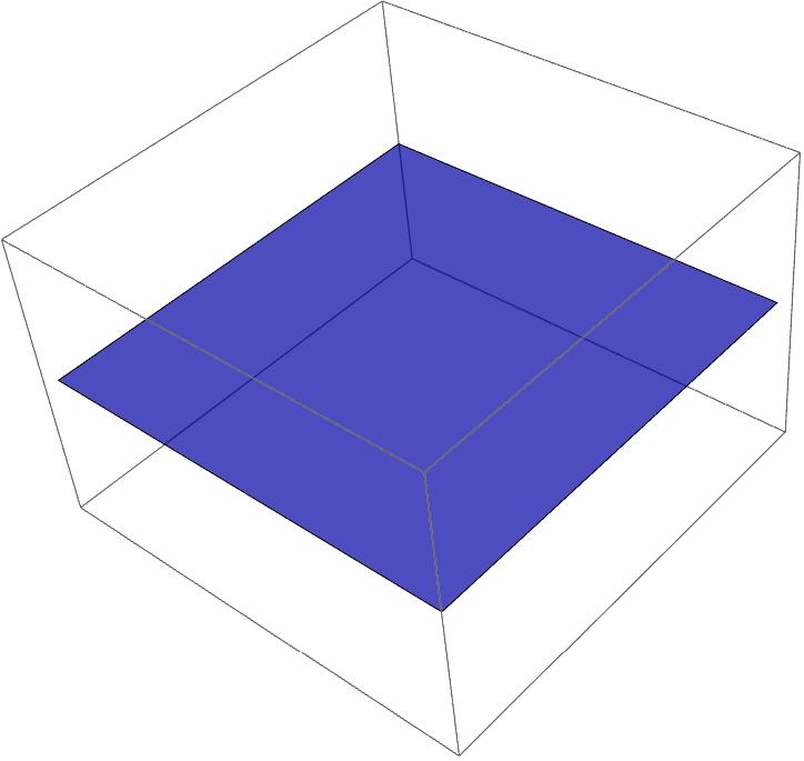
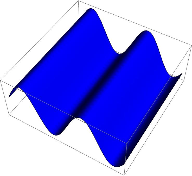
Figure 19 shows a simple surface. If it were truly 2D, we would not be able to see it. Figure 20 shows a wave. In a 3D volume of space-time, there are more 2D volumes of space-time in the wave.
But if we extrinsically warp the 2D surface into a wave, then the 3D volume contains more 2D spacetime. This is an increase in spacetime density in the 3D volume. That is, more low-dimensional spacetime is contained. This means that if we break away from the default of not using extrinsic deformation, then we have found a possibility for a recognizable space-time density.
The dimensional interface, which does not pass any geometric properties, but also due to the embedding, means that we can use an extrinsic deformation. We can recognize this expression in 3D. A pure wave representation cannot be recognized in 2D. It must always be via the space-time density. We still need something to combine it, but we will discuss that in part 3. For now, we have found a possible transition for mapping space-time density in 3D.
Wave mapping sounds like it’s going in the right direction for QFT. For QFT, we have to map the entire particle zoo of the Standard Model in low-dimensional space-time configurations. The possibility of extrinsic mapping is a start. However, this is never enough for the variety needed. It’s nice to know that something is still missing. But what is it? We have already looked at the solution twice and discussed it.
Drum roll, the solution is: the funnel. I’m leaving out the picture here, otherwise it wouldn’t have been a surprise. About the funnel in connection with the space-time boundaries, we came up with the idea that we can use an extrinsic mapping like the funnel. Question: Which object should the funnel map? Exactly, a black hole. What is a black hole? Right, the higher-dimensional transition. We need a mapping of a black hole in the lower-dimensional space. Then we have a higher-dimensional transition from 2D to 3D and are exactly where we want to be, in our space-time. It’s just stated here in the paragraph. Believe me, this simple idea was a difficult birth..
This black hole is also the reason for particles with rest mass. It is funny that there is a small calculation about a black hole in quite a few textbooks. Please calculate why an electron cannot be a black hole. The calculation is simple and results in a Schwarzschild radius of approximately 1.353\space *\space 10^{-57}. This is smaller than the Planck length. Thus, an electron cannot be a black hole. We will see later that this statement is absolutely correct for our spacetime. There is a minimal limit for the Schwarzschild radius. The electron is many orders of magnitude below that. But the electron is the perfect black hole in a 2D space-time. With a much smaller dimensional constant than in this space-time. Every space-time has its own Planck values. We already know the Planck mass of a simple 2D space-time, the rest mass of the electron.
The mystery of time certainly deserves more than just one section in this chapter. We can be sure that we will not solve this completely here either. We need a suitable logical description of time for the DP. This is discussed here because in the DP, time is only understandable in the context of the space-time boundary.
Time is always associated with a change. Without a change, no time could be recognized and vice versa. In the DP, everything we can recognize is associated with at least one spatial dimension. To map a density, we need at least one spatial dimension. A change in a mapping is therefore always a change in spatial dimension and time. Time and space are therefore not independent.
We have already started with an approach from the GR. Therefore, it is clear that we have to work with space-time as an inseparable object. However, it still makes sense to derive this unit as a consequence of density on the spatial dimension. Since space and time are not independent, we stick with space-time and space-time density.
But the question remains why time does not simply pass at a constant rate when the space density changes. This is because the change in the density of space is a change in the definition of space. Velocity is length divided by time. Time remains the same, but the length becomes “shorter” when accelerating. The object would slow down when accelerating. This does not correspond to observation. The calculations of GR only work because the time dimension has been made into a space dimension. Again: the time dimension in GR is the same as in SR, a space dimension with different signs. With the space dimension, the definition of geometry changes. Thus, the time dimension must also change as the definition of time. Space and time dimensions change the definition of what a unit of length or a unit of time is. Nothing is squeezed or stretched
Time is therefore bound to the space-time configuration. If this configuration changes, for example one dimension of space less, then this is no longer the identical space-time. The object space-time is left. Then time must also run towards zero. Therefore, each space-time configuration must have its own time dimension.
From this we can derive the following things for ourselves:
From the point of view of time, the space-time boundaries have been reached when it is no longer possible to achieve any effect on a state, no more change. Then you can no longer determine time. Let’s look again at the small formulas for effect and state in our space-time:
Effect h\space =\space l_P\space *\space m_P\space *\space c
State l_C\space *\space m_C\space =\space l_P\space *\space m_P
Let’s take only the right side in each case and put the effect in relation to the state:
\cfrac{state}{effect}\space =\space \cfrac{l_P\space *\space m_P}{l_P\space *\space m_P\space *\space c}\space \cfrac{1}{c}
This is the “resistance value” of space-time to change. This is bridged at c and there can be no more change. The effect from the low-dimensional must still be able to change the state mapping from the low-dimensional. This is the low-dimensional boundary.
From these considerations, we can equate time with the distance to the boundaries of space-time.
Time is a distance measure to the space-time boundary
Thus, in DP there is no flow of time or time arrow. The better way of looking at it is that experiencing time is the constant measurement of the distance to the space-time boundary. Therefore, there is no past. The next measurement at the boundary is always coming. The “measured value (the definition of the time unit)” can repeat itself from the past. But it is a different measurement. The flow of time is the series of distance measurements.
Finally, an often-asked question: Why is there only one time dimension? This question can be easily explained with our new perspective. You can leave the object space-time exactly once. Then you’re out. We can’t leave space-time again once we’re out. Therefore, there can only be one time dimension. The passage of time is the distance measurement to the space-time boundary. There is only one time dimension per space-time possible.
The idea that time is a measure of distance has another reason: the principle of relativity. This is a very good way of explaining a locally constant time. This will be worked through in the next chapter.