Everything consists of spacetime.
It should be common knowledge by now that QM can only generate a statement about the probability of the measurement result when predicting a measurement. As with uncertainty and entanglement, this is not incorporated as a basic concept. This only became apparent later. In fact, the Schrödinger equation was interpreted differently at the beginning. It was only the so-called Born probability interpretation (rule) that provided the solution. This made it clear that even though we have all the information about Schrödinger’s equation, nothing more precise than a probability can be derived from it. It is not as if further information needs to be collected in order to make an exact statement. In principle, it is not possible to obtain any information other than probability from QM.
We have already established that Einstein had his problems with entanglement. The probability interpretation was the second point. Einstein wrote to Max Born in 1926: “Quantum mechanics is very impressive. But an inner voice tells me that this is not the real Jacob. The theory provides a lot, but it hardly brings us closer to the mystery of the Old One. I am convinced that he does not play dice.” With entanglement, we arrive at a common solution between QM and Einstein. With probability, however, we must side completely with QM. We will see that, based on our approach, we can only obtain a probability.
Only with a special experimental setup can we obtain a clear statement about a measurement result. If we have determined a value in a measurement and then repeat this measurement immediately afterwards, we will obtain the identical measurement result again with 100% probability. We will explain why this is the case in the double-slit experiment. The “wave collapse” during measurement is not yet an issue here. The question here is why there are only probabilities and why these have a weighting.
For QM, we only need two basic elements for probability:
Whether the Schrödinger equation and thus probability is only a calculation or also a physical representation is a popular topic in interpretations of QM. We deviate from the Copenhagen interpretation and claim that probability clearly has a physical representation and is not just a mathematical quantity. This means that the two basic elements must have a direct representation in spacetime. However, this is different in terms of possibilities and weighting.
For the possibilities, we use the same basis as for superposition. In every n-dimensional spacetime volume of a spacetime density, there are infinitely many (n-1)-dimensional spacetimes and thus spacetime volumes and spacetime densities.
A single possibility cannot change itself. In cosmology, we have recognized that with only two spatial dimensions, we can only generate static images. In QM, we will later call these static images “stationary states” or “paths.” In cosmology, the creation of the image was a Big Bang; in QM, this is called “creation or destruction”. But then something changed in the 3D image due to an interaction. In 2D, everything remains static for the time being. When it comes to particles, these 2D images are called “virtual particles.” They exist but cannot be detected in 3D because the image is in 2D.
Important: There are always an infinite number of possibilities. This is clear in the example with the location in superposition. But what about spin? We only measure spin up and spin down. There are only two possibilities. We have to be careful here. With spin, too, the direction is always completely arbitrary. If we want to measure the spin, we choose a completely freely selectable axis for this measurement. Relative to this axis, the spin has the property of up or down. However, the measurement can refer to any direction (axis). Through the question/measurement we ask the system, we divide all possibilities into up and down. However, there remains an infinite number of possibilities.
During the measurement, we will then see that the possibilities can be mutually dependent. In the case of the double slit for the particles, this will result in the interference pattern. However, only very specific locations for the individual interactions are ever displayed on the screen. This means that only one possibility is ever “drawn” during the interaction. This is where the idea of wave-particle duality comes from. We will show that this dualism does not exist. A particle is a spacetime density with a volume and not a point. But a particle is also not a wave. The distribution and mutual influence are many different individual images. These low-dimensional images cannot be assigned a unique location in 3D. We do not need to explain wave-particle duality, as it does not exist in this form. In DP, we have a duality that is a simultaneous mapping in 3D and 2D. We have neither a point nor a wave. However, when we look at the weighting, we will see that the mathematical wave description is a very good analogy for this behavior.
There are two different types of weighting. In one type of weighting, the weighting depends on the properties of the particle, and in the other, it does not.
Let’s start with the example of spin, as it is simpler. With spin, there is actually no weighting. The fact that we always get a 50:50 probability of spin up and spin down is due to the question. All directions are present with identical weighting. By asking about spin up and spin down on a specific axis, we divide this set into two equal portions. The result should come as no surprise. However, this also means that spin must be a characteristic that belongs to the geometric features in 2D. We cannot distinguish these from 3D and they are always the same for us. This means that there is actually no weighting. Only the weighting that we introduce through the question.
Now let’s take our electron again, which we accelerate away from us. Here, things look different. The electron is very likely to follow a straight path. However, there is a small probability, which is not zero, that it will deviate from the straight path. The greater the deviation, the lower the probability. There are differences here. When I, as a human being, start moving in a straight line, I can confidently set the probability of deviation to zero. This is due to my mass, a special property of the object. At this point, I insist that this is only due to the very large ratio of my mass to that of the electron, as is the case with every other human being. Even if my wife would probably claim something different about my mass property.
Here, the weighting of probability is linked to a property, namely mass. However, mass is only one form of spacetime density. From superposition, we know that all possible 2D manifestations are separate 2D spacetimes. These must overlap spatially with the 3D spacetime density. Since all n-dimensional spacetimes are always continuous, there is an overlap at every point in our spacetime. This means that every point in spacetime would have the same weighting. Spacetime density now plays the decisive factor. We are more likely to find the electron where, in 3D, the 2D spacetime density best corresponds to the electron.
This means that, on average, the electron is most likely to be found where the 3D spacetime density is located. The images of the 3D and 2D spacetime densities overlap most strongly there. This is where wave imaging comes into play. We only have continuous spacetime. If we want to recognize something in 3D from 2D, we can do so almost exclusively via the extrinsic geometric characteristics in 2D. This makes wave mapping a good fit. The various geometric mappings in 2D can now be amplified or attenuated at certain locations in 3D. The electron will probably be most detectable at the locations where the amplification is greatest. However, we will clarify this in more detail with the double slit. On average, the probability for the electron is greatest exactly where the 3D spacetime density is located. Interference from the “waves” plays a role in the deviations.
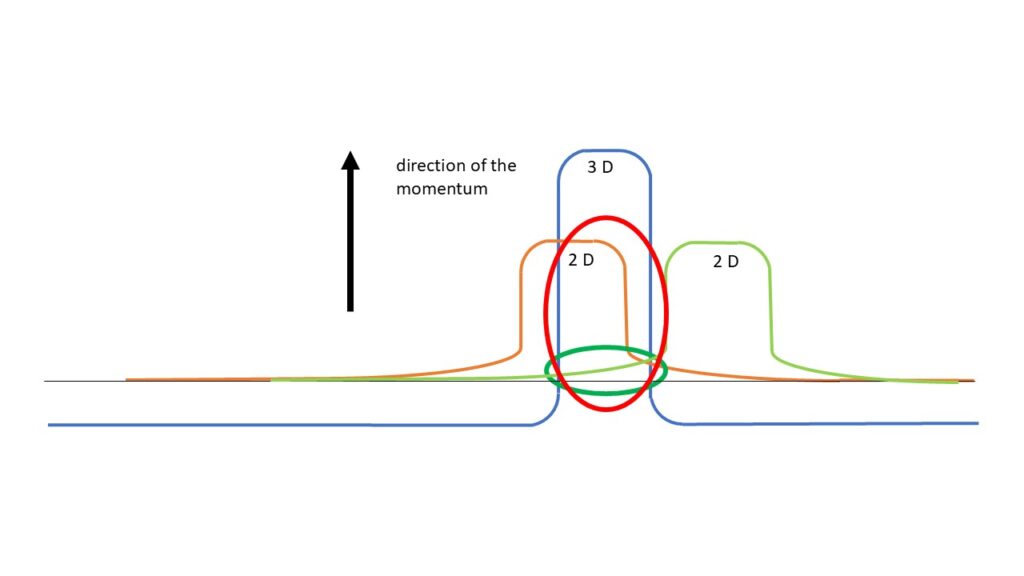
The amplitude represents the direction of the impulse. The wave on the left in orange has the largest intersection with the 3D spacetime density and is therefore more likely to be measured than the wave on the right in green. The intersections in the circles represent the probability.
In the image, we can see where the overlap in the 3D spacetime density is greatest. On average, this is where the particle will be most frequently encountered via an interaction from 2D. The greater the difference in wave amplitude, the lower the probability. Since the amplitude of the spacetime density in 3D is approximately a factor of greater for an object such as a human being than for an electron, the deviation is equivalent to zero. This is why we only perceive classical mechanics in everyday life and not quantum mechanics.
A good analogy for probabilities is an urn with balls. A damn big urn with an infinite number of balls. Well, there must be an advantage to being able to do theoretical physics.
In the case of spin, the balls in the urn are identical, with the difference being their color. Let’s say white and black. Then after many removals from the urn, we will have drawn an almost identical number of white and black balls.
In the case of the electron’s location, each spacetime point in 3D has a ball. The spacetime point with the greatest correspondence between the spacetime density of 3D and 2D has the largest ball. This makes it more likely to be drawn than another. However, the probability for the others is never zero. They are present in the urn. If the 2D spacetime densities influence each other, one ball becomes larger and the other smaller.
The wave image is somewhat simpler. If we reach into the urn from above, we are most likely to draw the spacetime density that has the greatest amplitude and thus reaches the highest point.
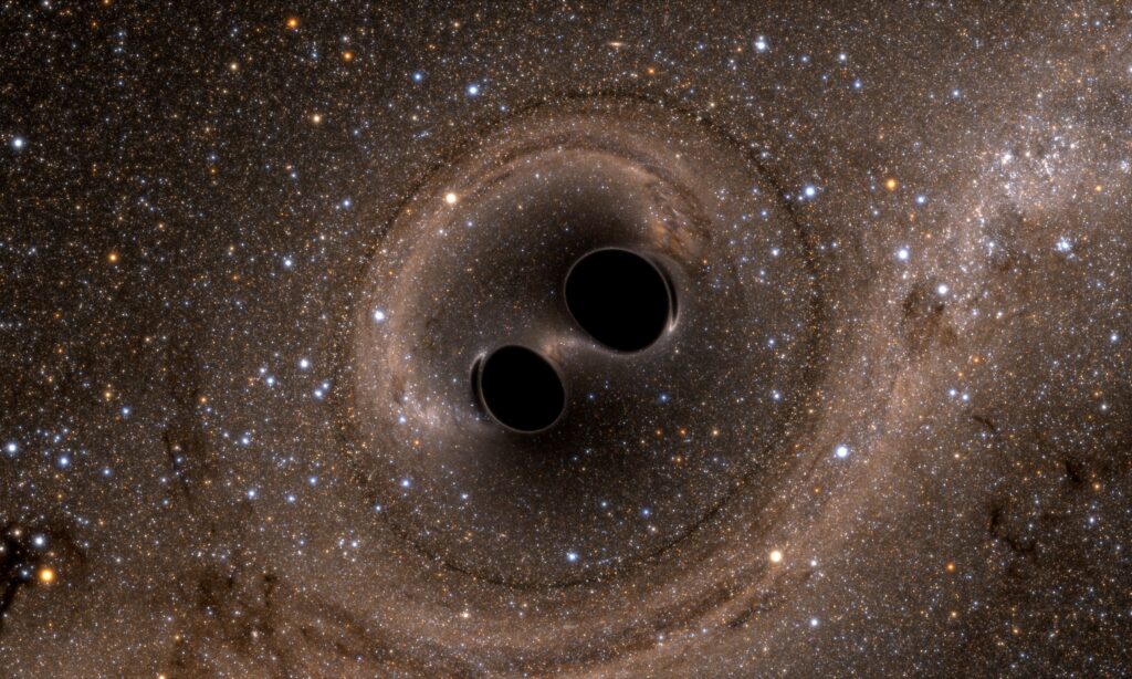
The argument about spacetime density helps with another case of probability. We will discuss the double-slit experiment later. This has already been done with larger objects. This is very well known for C60 buggy balls. A molecule consisting of 60 carbon atoms. Why do we not observe interference for 60 separate carbon atoms at the double slit, but rather for a C60 molecule? The probability of the location must be transferred to the entire structure and not to the components. In our example, we must move from electrons to humans.
The reason for this, as always, is spacetime density in continuous spacetime. This means that the spacetime density already overlaps in 3D, and we obtain a probability for the entire overlapping spacetime density in 3D.
We will see that this is also the reason why there can be such a thing as a “quasi-particle” in QM. You see, for QM to work, we simply cannot avoid continuous spacetime.
Here, it’s the same as with entanglement. The fact that we obtain a probability is already included in the approach to superposition. We have an infinite number of possibilities in the low-dimensional spacetime configurations. The surprise is rather why we can only ever obtain one of them in 3D. This is where our h with the interface comes into play. We only have energy from 3D spacetime density available. One possibility will interact with the measurement in 3D. Which one it will be cannot be determined in advance. That pretty much says everything there is to say about probability. We will discuss how the probabilities influence each other (the interference of the waves) in a later chapter on the mathematics of QM.
Our approach makes the often “strange” behavior of QM very easy to explain.